 It all started with a sundial.
Humans have depended on the predictability of heavenly bodies since the dawn of time. The Sun comes up in the morning and marches across the sky at the same rate every day. Long before man understood why that happened, he learned that the Sun's shadow could be used to mark time. Not so much on cloudy days, but we adapted to that, too.
 For a long time, it was good enough to organize the day into morning and
afternoon, or to break it up into hours and half-hours.
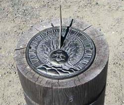
By and by, people
figured out how to build a sundial with enough precision to divide time into
minutes, or even finer. This large sundial is one of a pair at the Dodge
City (Kansas) train station – one each for Central and Mountain Time.
When the railroads implemented standard time zones in 1883, this was where
passengers gained or lost an hour. These dials are
42 feet across and can tell time to the
nearest minute. (There is a sundial in India, twice as big, with one-second
precision.)
For a long time, it was good enough to organize the day into morning and
afternoon, or to break it up into hours and half-hours.
By and by, people
figured out how to build a sundial with enough precision to divide time into
minutes, or even finer. This large sundial is one of a pair at the Dodge
City (Kansas) train station – one each for Central and Mountain Time.
When the railroads implemented standard time zones in 1883, this was where
passengers gained or lost an hour. These dials are
42 feet across and can tell time to the
nearest minute. (There is a sundial in India, twice as big, with one-second
precision.)
With this kind of accuracy, and with the development of high-quality clocks, it didn't take long to realize that something was not quite right. Four times a year, the Sun is directly overhead at local noon, but most of the time it's a few minutes early or late. What's that all about?
If the Earth's orbit were a perfect circle, and if its axis were upright in that orbit, Sun time and mechanical clocks would agree perfectly. We also would not have seasons, but that's another matter. The Earth moves faster in its orbit when it's closest to the Sun, which causes a small variation in the length of a day that cycles once throughout the year. The axial tilt causes additional variations that cycle between the equinoxes and the solstices, or twice a year. These two variations add up to produce differences between "sun time" and a regular clock, which can be plotted as the Equation of Time.
The Sun is almost never directly overhead at noon, either. The latitude where it's overhead at noon is plotted as the Declination of the Sun. Knowing this height, a mariner can tell his latitude if he can see the Sun at noon. If he also corrects for the Equation of Time and knows what time it is in Greenwich, England, when it's noon where he is, he knows the longitude as well. This is why a good chronometer was critical to oceanic navigation before modern electronic devices came along.
 Both of those equations depend on the same variable, the time of year. It's
useful to to remove this common parameter and plot one against the other.
Because they're periodic (repeating) functions, the resulting plot is
familiar to engineers as a Lissajous pattern. This special case is called an
analemma, after the Greek
ἀνάλημμα,
a support or
pedestal.
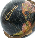
This figure is often found near a large sundial, so that
solar time can be reconciled to clock time. Because of its value in
navigation, it's also printed on globes – usually in the Pacific Ocean,
where it won't obscure land masses.
Both of those equations depend on the same variable, the time of year. It's
useful to to remove this common parameter and plot one against the other.
Because they're periodic (repeating) functions, the resulting plot is
familiar to engineers as a Lissajous pattern. This special case is called an
analemma, after the Greek
ἀνάλημμα,
a support or
pedestal.
This figure is often found near a large sundial, so that
solar time can be reconciled to clock time. Because of its value in
navigation, it's also printed on globes – usually in the Pacific Ocean,
where it won't obscure land masses.
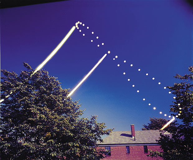
 If you stand on the exact same spot and observe the Sun's position (or
take a picture) at noon each day, it will describe this shape. The Sun will be
higher or lower in the sky as the seasons change, and there will be east-west
variations because of what drives the Equation of Time. This is true at
any time of day. A daily record of the Sun's position at the same time will
be an analemma, lower in the sky and tilted a bit because it isn't noon.
If you stand on the exact same spot and observe the Sun's position (or
take a picture) at noon each day, it will describe this shape. The Sun will be
higher or lower in the sky as the seasons change, and there will be east-west
variations because of what drives the Equation of Time. This is true at
any time of day. A daily record of the Sun's position at the same time will
be an analemma, lower in the sky and tilted a bit because it isn't noon.
The analemmas in the figure at left are what would be seen from the spot where I chose to record for this project. The tilts vary with latitude. At the Equator, the analemma is horizontal throughout the day. As the viewer moves north or south from there, the patterns shift until they are all nearly vertical at the Arctic or Antarctic Circle.
Some of the images for this article are too big to display inline, so they are represented by thumbnail images with a red border. Click the thumbnail to see the image full-size. The large image will pop up in a new window, in some cases large enough that you have to scroll it to see it all.
 I'm certainly not the first one to photograph this pattern, and neither am I
the first to write about it. Here are stories of some other analemma
projects, and the beautiful results that came out of them.
I'm certainly not the first one to photograph this pattern, and neither am I
the first to write about it. Here are stories of some other analemma
projects, and the beautiful results that came out of them.
Dennis di Cicco, an amateur astronomer and editor at Sky & Telescope, photographed The First Ever Analemma in 1978-79. He described the process in the June 1979 issue of that magazine, which is reproduced here. He used a 4×5 graphic camera with a digital alarm clock to trip the shutter at precisely the right time on the days he wanted sun shots. As the article describes, it was a lot more work than it sounds like.
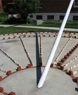
Frank Zullo, a pro photographer in Carefree, Arizona: Photographing the Analemma. He recorded the sun with a dedicated camera mounted at his house in 1990-91, and superimposed it onto a beautiful picture of America's largest sundial.
Pál Váradi Nagy, a software developer in Transylvania: Analemma of Kolozsvár City. He shot his analemma and background scene from a public site, so he couldn't leave a camera in place. He made a fixture that he carried to the site several dozen times over the course of a year, 2012-13.
Anthony Ayiomamitis, astrophotographer in Athens, Greece: Solar Image Gallery – Analemma. Several images, 2002-4. The backgrounds are ancient Greek temples.
Tunç Tezel, an amateur astronomer in Turkey: The Making of a Tutulemma. He chose the time of day so that his analemma would include a totally eclipsed Sun in March 2006.
György Bajmóczy, a photographer in Hungary: Traces of the Sun. This two-minute video was made from 116,000 still shots taken at different times of day throughout the year. It shows dramatically how the analemma is formed, and how it moves across the sky from sunrise to sunset.
The analemma at noon would be a fairly boring scene in Connecticut. Because of the Sun's elevation, there would be nothing in the background but sky. Accurate, but boring. The Sun's position in morning or evening at least lets the camera include some features on the surface. It shouldn't be too early or late, lest the Sun be below the horizon at the chosen time. After minimal headscratching, I decided on a time about fifteen minutes before the winter sunset. That's about as low in the sky as I wanted the Sun, so it wouldn't be hidden behind a tree or something. Now it remained to find a suitable background. One thing you quickly notice when sifting through the images of others, is that the best ones are on hilltops like the Acropolis in Athens. That lets the photographer get close to his scene, but there are no trees in the way of the area where the analemma will form.
Scouting a few local places, I was looking for a scene with a lot of open sky behind it. The analemma would need unobstructed space from the horizon up to 35° elevation. I decided to record at the Bridgeport (Conn.) airport, since I've spent a lot of time there over the past thirty years. But where to place the camera on the airport? Here's the layout I came up with, chosen for the location of some local flying landmarks as well as placement of the analemma. I rejected other locations around the airport because
I also decided to compose a panoramic shot that includes just about everything in front of the camera. This presented some interesting challenges, especially in representing the scene without distorting it.
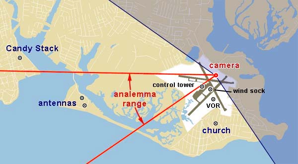
Google Maps made it easy to find a good spot for the camera. I used its "what's here" function to get latitude and longitude for each of these landmarks, as well as for several possible camera locations. They provide this information to six decimal places of precision. That's one millionth part of a degree, which works out to four inches. I wonder if it's really that accurate. I know my mouse pointer isn't.
Here's the scene, one-half actual size. As you can see in the map above, the field of view is about 150°. The top of the image is seven degrees above the horizon. We're going to need five times that much to include the summer sun at the chosen time of day, so you can see that this will be a rather large picture by the time it's finished. As you scroll from left to right, you can find the landmarks I wanted to include.

 The spire of the Lordship Community Church pokes up above the trees. When
dinosaurs roamed the Earth, there was an office of the National Weather
Service on the airport. A living human would go outside every hour to observe
the weather. If it was very foggy, he looked for that church spire, which
was the official marker for 5/8 mile
visibility. The NWS observer is long gone, but 5/8 miles remains as the
official discriminator between "fog" and "mist."
The spire of the Lordship Community Church pokes up above the trees. When
dinosaurs roamed the Earth, there was an office of the National Weather
Service on the airport. A living human would go outside every hour to observe
the weather. If it was very foggy, he looked for that church spire, which
was the official marker for 5/8 mile
visibility. The NWS observer is long gone, but 5/8 miles remains as the
official discriminator between "fog" and "mist."
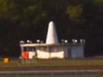 The Bridgeport VOR. We used to drive past one of these on the way to Scout
camp. Nobody seemed to know what it was, but it had an FAA sign on the fence
so we figured it had something to do with airplanes. It generates a signal
that lets the pilot know his magnetic bearing from this point, so he can navigate any
line that passes through it. This one also has
DME equipment that drives a
display in the plane to show distance. With both pieces of information, the
pilot can tell his exact location. This unit will eventually be
decommissioned as GPS slowly becomes our sole means of electronic navigation
in the USA.
The Bridgeport VOR. We used to drive past one of these on the way to Scout
camp. Nobody seemed to know what it was, but it had an FAA sign on the fence
so we figured it had something to do with airplanes. It generates a signal
that lets the pilot know his magnetic bearing from this point, so he can navigate any
line that passes through it. This one also has
DME equipment that drives a
display in the plane to show distance. With both pieces of information, the
pilot can tell his exact location. This unit will eventually be
decommissioned as GPS slowly becomes our sole means of electronic navigation
in the USA.
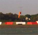 It wouldn't be much of an airport without a wind sock. The orange and white
things on the ground are laid out in a
100-foot diameter segmented circle,
to make it easy to find the wind sock from above.
It wouldn't be much of an airport without a wind sock. The orange and white
things on the ground are laid out in a
100-foot diameter segmented circle,
to make it easy to find the wind sock from above.
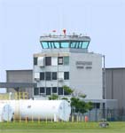 There are 14,000 registered airports in the United States. 5000 of them
have paved runways. 516 of those have control towers, but many
people think it's not really an airport unless it has a
control tower. The Bridgeport airport is one of the 3½% with a tower, and
here it is. It's right out in the middle of the place, and it would be hard
to imagine this airport without it, even though there's not much traffic to be
controlled these days.
There are 14,000 registered airports in the United States. 5000 of them
have paved runways. 516 of those have control towers, but many
people think it's not really an airport unless it has a
control tower. The Bridgeport airport is one of the 3½% with a tower, and
here it is. It's right out in the middle of the place, and it would be hard
to imagine this airport without it, even though there's not much traffic to be
controlled these days.
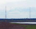 The WICC antennas are a commonly-used reporting point. They're two miles
from the airport, right base for 11 or left base for 6.
The callsign is a throwback to an era long departed: WICC stands
for the Industrial Capital of Connecticut, a reminder of
a time when Bridgeport had several busy factories.
The WICC antennas are a commonly-used reporting point. They're two miles
from the airport, right base for 11 or left base for 6.
The callsign is a throwback to an era long departed: WICC stands
for the Industrial Capital of Connecticut, a reminder of
a time when Bridgeport had several busy factories.
 This place is on 3-mile final for Runway 11. It's the United Illuminating
generating station, which could burn either coal or oil until recently. Now
the oil tanks have been removed and
it burns only coal, and it only does that for a few days each year. It's cheaper
to import electricity from hydro plants in northern Québec. Because of
the bright paint job, this is known to local pilots as the Candy Stack.
There's another smokestack almost the same size nearby. It's in the picture
between the WICC antennas and the Candy Stack, but I make no particular
reference to it because it's not used as a local reporting point, and it
isn't painted.
This place is on 3-mile final for Runway 11. It's the United Illuminating
generating station, which could burn either coal or oil until recently. Now
the oil tanks have been removed and
it burns only coal, and it only does that for a few days each year. It's cheaper
to import electricity from hydro plants in northern Québec. Because of
the bright paint job, this is known to local pilots as the Candy Stack.
There's another smokestack almost the same size nearby. It's in the picture
between the WICC antennas and the Candy Stack, but I make no particular
reference to it because it's not used as a local reporting point, and it
isn't painted.
In the age of digital photography, we are fortunate that it doesn't take a whole year to find out whether a project like this failed or succeeded. Forty years ago, Dennis di Cicco had to mount a dedicated camera rigidly n place, and make several dozen exposures on a single emulsion. Then he had to develop it carefully, and hope nothing went wrong. In fact, something did go wrong the first time, and he had to wait another year before he got the result he published in 1979.
Now, we can make the background image at any time. We can even make several of them, and choose a favorite. The sun images are individual shots that are added digitally to the background. The dedication and planning needed for the film analemmas is hard to imagine in the early part of the 21st century.
Once I chose a background scene, all I had to do was record it on a picturesque day. This can't be done at the same time of day as the sun shots, because the scene would be backlit. The best choice is early in the day (we're looking westward at the scene), with low humidity to bring out the blue of the sky. Even di Cicco acknowledged this problem, and nobody was bothered by that. Then, I need to be careful that the sun shots are pasted in the correct place on the background scene. To do that, I derived pixel-mapping equations for a scene that was projected onto a cylindrical "film" 20 millimeters from the convergence point. You saw the result of this process in the panorama already shown, and didn't think twice about it.
For this project I chose an effective focal length of 20mm, which kept the image height to ten inches. This led to these pixel-mapping equations for azimuth (φ) and elevation (θ), which I used to put the suns in the correct position on the background scene:
If you really want to see how this was derived (it's a long story), click here.
Don't want to see the math? Click here.
 I mentioned earlier that I was going for a field of view about 150°.
To get that kind of coverage with the sensor in my camera (24mm wide) would
require a 3mm lens! This is the kind of fisheye effect you see in
apartment-door peepholes –
certainly, not the effect I was looking for. I took a different approach,
using the stitch-panorama technique that is quite common in this age of
digital photography. But it was necessary to understand how to map locations
in the scene to pixels in the image. To explain that, let's step back and
take a look at an alternate way to understand how a lens produces images. In
the usual presentation, we see how a thin lens makes an image on a plane
located some distance behind it. The image is inverted, but we're smart
enough to turn the film around when we look at it.
I mentioned earlier that I was going for a field of view about 150°.
To get that kind of coverage with the sensor in my camera (24mm wide) would
require a 3mm lens! This is the kind of fisheye effect you see in
apartment-door peepholes –
certainly, not the effect I was looking for. I took a different approach,
using the stitch-panorama technique that is quite common in this age of
digital photography. But it was necessary to understand how to map locations
in the scene to pixels in the image. To explain that, let's step back and
take a look at an alternate way to understand how a lens produces images. In
the usual presentation, we see how a thin lens makes an image on a plane
located some distance behind it. The image is inverted, but we're smart
enough to turn the film around when we look at it.
It is completely equivalent to analyze this situation as if we're projecting the image onto a plane located the same distance in front of the lens plane, as in the second sketch above. This is a common construct in describing how maps are made, and it offers the advantage of letting us think about an upright image.
Imagine if we had our sensor wrapped around something like a coffee can. In the vertical dimension, it's normal. But around the horizon, we're projecting onto a cylinder. By comparison to the image above, we see that the radius of the cylinder is equivalent to the focal length of the lens. I chose 20mm for this focal length, for reasons related to the size of the finished image.
By generating the image this way, we find that azimuth (bearing from the camera) maps directly to pixel count. Elevation requires the usual trigonometry because that dimension is flat, not circular. There are some approximations, but I found them acceptable because the objects in the scene were thousands of feet away from the camera. For instance, I assumed
There are still people who agree with the first assertion, and the second one keeps the math simple. Elevation maps in a simple way to pixel count (zero is at the top of the frame):
where θ is elevation above the horizon, and y0 is the pixel number that represents the horizon. n is the focal length, expressed in pixels. That is,
δ: pixel pitch (5.5μm)
f: focal length (20mm)
Horizontally, we have
where φ is the azimuth angle and x0 is a pixel value that corresponds to true north. To get m, we realize that the circumference of the cylinder is
where m is the ratio of pixels to degrees. It is also related to the radius of the projection surface, which is the focal length:
Combining eqs. 4 and 5,
In a stitch-panorama, the projection surface isn't really a cylinder. It's a series of planes, one for each rotation of the camera. But if there are enough of these planes, and they are thin enough, the approximation to a smooth surface is good enough. In practice, I found that the mapping is adequate. The azimuth, which I can measure, is accurately located within two or three pixels, over a picture that's several thousand pixels wide.
 How good is this approximation? Let's say we're imaging with a field of view
whose angle is 2α. We're mapping half of this field onto
m⋅α pixels according to eq. 3. In reality, the number of
pixels in half the field is
How good is this approximation? Let's say we're imaging with a field of view
whose angle is 2α. We're mapping half of this field onto
m⋅α pixels according to eq. 3. In reality, the number of
pixels in half the field is
h = f tan(α)
which is a slightly larger number. Eq. 3 uses the small-angle approximation
tan(α) ≅ α
where α is expressed in radians. The error in this approximation is
ε = (tan(α) / α) - 1
That error is 0.25% for a field of view whose half-angle is 5°, which is quite acceptable. In other words, if we take a new slice of panorama every ten degrees, the error will not be perceptible.
So there we have it. Eqs. 1 and 3 are the mapping equations, and eqs. 2 and 6 give the proportionality constants. Now we have enough information to combine the sun shots for the analemma with the background scene. To repeat and summarize, the conversion from azimuth and elevation to pixels in the scene is
derived from the pixel pitch of the sensor and the focal length of the lens.
The astute reader will have noticed that the parameters 3636 and 63.467 in those equations are related by the factor 180/π, the same relation as between degrees and radians. This is not a coincidence. It's because the horizontal aspect of the image comes from a projection onto a cylindrical surface, which eliminates the trigonometry we need to make the vertical part work. In other words, the "small angle approximation" is valid for all angles, and it's not approximate in this case.
How big is the Sun? It's 93 million miles away on average, and 864,576 miles in diameter. Dividing one number by the other (and taking the inverse tangent if you don't like the small-angle approximation), we see that our star subtends about half a degree from an Earthly viewpoint. Using the factor from Eq. 6, that works out to 32 pixels for an image made by a 20mm lens on the sensor used for this project.
In keeping track of all this project's components, it's crucial to do things at the right time. Daylight Time can be a nuisance in this regard, so I decided early on to do all my record-keeping in Universal Coordinated Time (UTC) ‐ also known to pilots as "Zulu Time" because its time-zone designator is Z. This is the time at the Royal Observatory in Greenwich, England (London), five hours different from Eastern Standard Time (where I live). It stays put when we change our clocks in the Spring and Fall, making it more practical for any events related to what time a sundial would show. 1400Z is
My camera (and its operator) are not too good about changing the clocks either, so I've set the camera to Zulu Time. If you look at the EXIF data in any of the images on this page, that is what you will find.
If you were to record a noontime analemma that changed its "clock" twice a
year, it would look like this:

Not very elegant at all.
 In a later section, I explain how it's not possible to
image the Sun and the scene correctly at the same time. But I was able to
make a series of calibration shots through a
64X neutral density filter to
test the calibration of the pixel-mapping equations. This kept the Sun from
blowing out completely, but left the rest of the image almost completely
black. There was enough information in that deep shadow to locate structures
in the scene by manipulating the contrast in Photoshop. This image shows
what these images look like, with the original scene on the right and the
lightened scene on the left. The Sun is still badly overexposed, but there
is enough definition to locate its center, which is what we need to calibrate
the pixel map.
In a later section, I explain how it's not possible to
image the Sun and the scene correctly at the same time. But I was able to
make a series of calibration shots through a
64X neutral density filter to
test the calibration of the pixel-mapping equations. This kept the Sun from
blowing out completely, but left the rest of the image almost completely
black. There was enough information in that deep shadow to locate structures
in the scene by manipulating the contrast in Photoshop. This image shows
what these images look like, with the original scene on the right and the
lightened scene on the left. The Sun is still badly overexposed, but there
is enough definition to locate its center, which is what we need to calibrate
the pixel map.
It's not important to take the calibration pictures at exact analemma time – just to know when they were taken, and the Sun's azimuth and elevation that can be read from NOAA's Solar Position Calculator. If this matches the pixel mapping equations, we're all set. If not, there's something wrong with the theory.
Fortunately, the match was within tolerance. It's necessary to understand what that tolerance is. The Earth rotates 360° every 1440 minutes. Dividing one number by the other, we see that the Sun moves one degree every four minutes. It subtends about one-half degree in the sky, which is to say that it takes only two minutes to move through its own diameter. This is dramatically obvious at sunset, but it's true for the rest of the day, too.
The details of the calibration are in a separate article.
 Since I was already committed to a Photoshopped image, it seemed like it
would be fun to include the
solar eclipse of 21 August 2017. Connecticut wasn't in the path of
totality – the Sun was only 69% obscured here, so even at the center of
the event, there was still a healthy crescent showing. The problem for me
was that maximum obscuration in Connecticut happened an hour and a half
before my analemma time. Throughout the event, the Sun was much higher in
the sky than the highest of my analemma sun shots. To image it faithfully,
I'd have to more than double the height of the picture, which was already
almost all blank space.
Since I was already committed to a Photoshopped image, it seemed like it
would be fun to include the
solar eclipse of 21 August 2017. Connecticut wasn't in the path of
totality – the Sun was only 69% obscured here, so even at the center of
the event, there was still a healthy crescent showing. The problem for me
was that maximum obscuration in Connecticut happened an hour and a half
before my analemma time. Throughout the event, the Sun was much higher in
the sky than the highest of my analemma sun shots. To image it faithfully,
I'd have to more than double the height of the picture, which was already
almost all blank space.
So I re-scheduled the eclipse in software. I took a picture of the Sun every five minutes while the Moon was in transit, and used NASA's solar position calculator to relocate each image to where it would be if the moment of totality were the same as the analemma time. I hope you don't mind the manipulation – I'm not really trying to trick anyone, just remembering a sideline view of the Great American Eclipse.
Light meters don't work when the subject is our nearest star. It's just too bright. If you want anything resembling a normal exposure, you have to calculate it, or find it by trial and error. Fortunately, the brightness of the Sun doesn't change, so this isn't hard to do. The calculation yields numbers that no ordinary camera can provide, so the usual procedure is to shoot through a very dark filter.
This is another section with a lot of tech-speak and many equations. if you
want to see it anyway,
Click here.
Otherwise, just get 14 or 15 f-stops worth of neutral density filters and use
or something equivalent.
Don't want to see the math? Click here.
 The goal of most exposure systems is to produce an image with a wide range of
brightness values. They should approach the pure-black and pure-white ends
of the histogram without bunching up there; and the average scene values
should center on the mid-values of the histogram. A well-calibrated spot
meter will produce a centered histogram if it's aimed at a standard grey
card.
The goal of most exposure systems is to produce an image with a wide range of
brightness values. They should approach the pure-black and pure-white ends
of the histogram without bunching up there; and the average scene values
should center on the mid-values of the histogram. A well-calibrated spot
meter will produce a centered histogram if it's aimed at a standard grey
card.
That's a fairly basic statement of what an automatic camera tries to do with an average scene. More specifically, it will try to set the exposure so the average luminance of the scene is in the middle of the histogram, what is often called Zone V. To help photographers discuss things like this, they have a logarithmic system of Light Values, defined as
LV = log2 (L S / K)
where
L: luminance, candela / m², an average value for the scene
S: ISO sensitivity
K: exposure factor (12.5 for Nikon and Canon digital cameras)
log2 means the base-2 logarithm. If you don't have a calculator that does that kind of math,
log2 (x) = log(x) / log(2) = 3.32 log(x)
Obviously, it's important to find the "correct" measure of luminance for the scene. A lot of electrons and ink have been spilled over just what that means. For our purposes, let's just say that if you can measure L, you've defined Zone V. With spot metering, a photographer can get pinpoint control over the lightness value of the pixels in his digital image.`
By convention, the standard exposure value is determined for ISO = 100, for which LV = EV.
EV = log2 (N² / t)
where
N: ratio of focal length to aperture diameter, commonly known as
F-number
t: exposure time (seconds)
Because these numbers are defined by base-2 logarithms, each unit represents twice or half the light of its neighbor. This is convenient for adjusting the camera, because exposure times and F-stops generally work the same way.
If ISO is different from 100, the exposure value is adjusted accordingly. By lucky coincidence, each unit of EV is roughly equivalent to one step in the Zone System, and most images can accommodate ten or eleven of them. Here are some typical light values that we might find in everyday life.
Well, we were doing OK until that last one. Most camera exposure meters can handle scenes up to about LV = 21, but the Sun is completely out of range. So we introduce neutral density filters, and quickly find that we need at least 13 F-stops' worth, which will reduce the Sun's apparent luminance to LV 21.
The Sun is a very bright object, and we don't really want it averaged to Zone V; so we can afford to bump the calculated value by at least two or three EV (F-stops). That is what has been done here. I stacked two ND filters, 64X and 400X. For ISO 100, this reduced the Sun's luminance to
LV = (1.6 × 109 × 100 / 12.5) - log2 (64 × 400)
= 33.6 - 14.6 = 19
 EV 19 would place the Sun at Zone V, which would be kind of dreary.
Opening up two stops to EV 17, we arrive at this exposure:
EV 19 would place the Sun at Zone V, which would be kind of dreary.
Opening up two stops to EV 17, we arrive at this exposure:
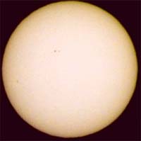
which worked rather well. Here is the resulting image, after removing the strong color cast from the neutral density filters.
 This is the histogram of that image. The Sun is mostly very bright, but
there is enough low-level detail to show some small sunspots that were
visible that day. There are no pixels bunched up at the far right side
of the histrogram, meaning that no part of it is overexposed.
This is the histogram of that image. The Sun is mostly very bright, but
there is enough low-level detail to show some small sunspots that were
visible that day. There are no pixels bunched up at the far right side
of the histrogram, meaning that no part of it is overexposed.
In a thoroughly helpful astronomy workshop monograph, Sakari Ekko recommends an exposure
t = (N² D) / (S K)
where
D = density reduction (e.g., 64 × 400)
K = 70 × 106, representing the Sun's luminance
and the other parameters are as already defined. This works out to about LV 18, which would push the histrogram one stop to the left. This is still quite usable, but I would prefer not to have the compressed dynamic range.
All of the sun shots were exposed by this method, reduced to a size appropriate for a 20mm lens (32 pixel diameter), and added to the basic scene at locations calculated by the pixel-mapping equations in an earlier section of this article. I wish I could have made the sun images larger, but then I'd have needed a rather large wall to display the whole picture.
 The final picture is about
!!## 10,000 × 3000 pixels, which prints
33 inches wide and 10 inches high.
Except for the analemma and time-shifted eclipse, all of the detail is in a
one-inch band at the bottom, which was introduced
early in this article.
Some of it is repeated here at the end, full size.
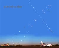
The whole image is posted on
Flickr. The crop at right is about one third of it, showing how the 2110Z
Sun spent a year between the airport's control tower and the Candy Stack.
The final picture is about
!!## 10,000 × 3000 pixels, which prints
33 inches wide and 10 inches high.
Except for the analemma and time-shifted eclipse, all of the detail is in a
one-inch band at the bottom, which was introduced
early in this article.
Some of it is repeated here at the end, full size.
The whole image is posted on
Flickr. The crop at right is about one third of it, showing how the 2110Z
Sun spent a year between the airport's control tower and the Candy Stack.

anon., Solar Position Calculator, NOAA, Washington, D.C.
di Cicco, Dennis, "Exposing the Analemma," Sky & Telescope 57(6):536, June 1979.
Ekko, Sakari, Photographing the Sun, European Assn. for Astronomy Education, Turku, Finland.
Sobel, Dava, Longitude, Fourth Estate, London, 1995.